Intro to Variational AutoEncoder

Variational Autoencoders
1. Intro Suppose we accumulate the dataset whose underlying (unknown) true distribution is characterized by \( p^{*}(\mathbf{x}) \) where \( \mathbf{x} \) is high-dimensional vector. Generally we will never realize such \( p \) in any exact analytical form for real application. So we resort to approximate to function \( p_{\theta }(\mathbf{x}) \) parametrized by \( \theta \), meaning that we aim to minimize some distance between \( p_{\theta } \) and \( p^{*} \). Often we are interested in conditional version of the model \( p_{\theta }(\mathbf{x} |\mathbf{z}) \) as oppose to just \( p_{\theta }(\mathbf{x}) \). This variable is refer to as latent construct which is the unobservable process shared among data point (latent is not part of the dataset). Our interest is to find the marginalized likelihood \( p_{\theta }(\mathbf{x}) \) which involve integrating out over all latent variable \( \mathbf{z} \). This is the intractable problem as \( \mathbf{z} \) is never know and the high-dimensionality nature, so we have no analytical formula. If we use normal Guassian or discrete categorical distribution, analytical marginal form exists. However, we often aim to compute complex function, e.g. video or image generation. This also means that the posterior \( p_{\theta }(\mathbf{z} |\mathbf{x}) \) will also be intractable as this is linked by

\[ \mathnormal{p_{\theta }(}\mathbf{z|x}\mathnormal{) =\frac{p_{\theta }(\mathbf{x,z})}{M}}\text{\ ,\ where} \ M=\ p_{\theta }(\mathbf{x}) =\int _{z\in Z} p_{\theta }(\mathbf{x} ,\mathbf{z}) d\mathbf{z} \]

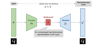
Since \( p_{\theta } \) will never be known, we resort to approximate \( q_{\theta } \) which is typical Universal function approximator like Neural Network. Variational AutoEncoder (VA) operates with closed framework to generic AutoEncoder (AE). Roughly speaking, AE comprises two main structure: encoder \( g_{\alpha } \) whose function is to compress original data input \( \mathbf{x} \) to some lower-dimensional latent representation \( \mathbf{z} \), and the decoder \( w_{\omega } \) whose job is to project this compressed version of inputs \( \mathbf{z} \) back to original inputs \( \mathbf{x}^{*} =w_{\omega }( g_{\alpha }(\mathbf{x})) \) while minimizing the reconstruction error typically via Euclidean distance loss. Some variant to this is Denoising AE where the original inputs are partially corrupted though random perturbation before feeding the encoder to avoid overfitting. Contrary to AE, VA is rooted from the method of graphical model:

\[ p_{\theta }(\mathbf{z} |\mathbf{x}) =p_{\theta }( z_{0} ,z_{1} ,...|\mathbf{x}) =p_{\theta }( z_{< N} |\mathbf{x}) =\prod{}_{n\in N} p_{\theta }( z_{n} |\mathrm{Parent}( z_{n}) ,\mathbf{x}) \]

Where each term is conditioned by parents of \( z_{n}\). Instead of mapping the vector input into a fixed point, VA map it to some distribution while retaining the encoder-decoder structure. We never know each term in the product, rather we try to find \( q_{\lambda } \approx p_{\theta } \). Suppose that we have true optimal parameter

\[ \ \lambda ^{*} =\arg\max_{\lambda }\prod{}_{n\in N} q_{\lambda }(\mathbf{x}_{n})\rightarrow \arg\max_{\lambda }\sum{}_{n\in N}\log q_{\lambda }(\mathbf{x}_{n}) \]

which maximize the probability of seeing the true sample set from the model \( q_{\lambda } \), we first sample \( \mathbf{z} \) from prior distribution \( q_{\lambda ^{*}}(\mathbf{z}) \) in the \( \mathbf{z} \)-space, e.g. \( z\sim \mathcal{N}( 0,1) \), after that the value of \( \mathbf{x}_{n} \) is generated by conditional \( p_{\theta }(\mathbf{x|z}) \). This conditional defines the generative process, similar to decoder \( w_{\omega } \) that map latent space to data space. Similarly, we also have probabilistic encoder or posterior that decode the latent variable \( p_{\theta }(\mathbf{z |x}) \), and we already have seen that this quantity is impractically to obtain. We first write the evidence of the observed variables, \( \log p_{\theta }(\mathbf{x}) \) as

\[ \log p_{\theta }(\mathbf{x}) =\log p_{\theta }(\mathbf{x})\int _{\mathbf{z}} q_{\lambda }(\mathbf{z|x}) d\mathbf{z} =\log\int _{\mathbf{z}} p_{\theta }(\mathbf{x} ,\mathbf{z}) d\mathbf{z} = \]

\[ \log\int _{\mathbf{z}} q_{\lambda }(\mathbf{z|x})\frac{p_{\theta }(\mathbf{x} ,\mathbf{z})}{q_{\lambda }(\mathbf{z|x})} d\mathbf{z} =\log\mathbb{E}_{\mathbf{z} \sim q_{\lambda }(\mathbf{z|x})}\left[\frac{p_{\theta }(\mathbf{x} ,\mathbf{z})}{q_{\lambda }(\mathbf{z|x})}\right] \geqslant \mathbb{E}_{\mathbf{z} \sim q_{\lambda }(\mathbf{z|x})}\left[\log\frac{p_{\theta }(\mathbf{x} ,\mathbf{z})}{q_{\lambda }(\mathbf{z|x})}\right] \]

\[ =\mathbb{E}_{\mathbf{z} \sim q_{\lambda }(\mathbf{z|x})}[\log p_{\theta }(\mathbf{x} ,\mathbf{z})] -\mathbb{E}_{\mathbf{z} \sim q_{\lambda }(\mathbf{z|x})}[\log q_{\lambda }(\mathbf{z|x})] \]

\[ =\mathbb{E}_{\mathbf{z} \sim q_{\lambda }(\mathbf{z|x})}[\log p_{\theta }(\mathbf{x} ,\mathbf{z})] + H[ q_{\lambda }(\mathbf{z|x})] \ =L \]

where \( H\) is the entropy, describing the uncertainty of variational distribution \( q_{\lambda }(\mathbf{z|x}) \). When maximize \( \log p_{\theta }(\mathbf{x}) \), the first expectation is the weighted average over all possible value of \( \mathbf{z} \) with weight \( q_{\lambda }(\mathbf{z|x}) \), and the natural choice of \( q_{\lambda }(\mathbf{z|x}) \) that maximize \( \mathbb{E}_{\mathbf{z} \sim q_{\lambda }(\mathbf{z|x})}[\log p_{\theta }(\mathbf{x} ,\mathbf{z})] \) would be the distribution that put all its weight to the largest fixed data point \( \mathbf{z} \), which is what Dirac Delta distribution exactly does. It put weight of 1 to largest \( p_{\theta }(\mathbf{x} ,\mathbf{z}) \), and 0 for the raise of data point. However, this becomes problematic when consider the second term, the entropy of this distribution \( q_{\lambda }(\mathbf{z|x}) \) represents no uncertainty, e.g. approaching \( -\inf \)(This can be seen by consider Gaussian \( x\sim \mathcal{N}( x_{0} -\mu ,x_{0} +\mu ) \), then as \( \mu \rightarrow 0 \), the entropy \( \mathbb{E}_{x}[ 1/p( x)] =\log( 2\mu )\xrightarrow{\mu \rightarrow 0} -\inf \)). In other word, when maximizing the evidence \( \log p_{\theta }(\mathbf{x}) \), we want to have distribution that fit to the peak of joint distribution but also spread as wide as possible, e.g. high entropy. The objective \( L \) is called evidence lower bound (ELBO), which can be rewritten as

\[ L =\mathbb{E}_{\mathbf{z} \sim q_{\lambda }(\mathbf{z|x})}\left[\log\frac{p_{\theta }(\mathbf{x} ,\mathbf{z})}{q_{\lambda }(\mathbf{z|x})}\right] =\mathbb{E}_{\mathbf{z} \sim q_{\lambda }(\mathbf{z|x})}\left[\log\frac{p_{\theta }(\mathbf{x|z}) p_{\theta }(\mathbf{z})}{q_{\lambda }(\mathbf{z|x})}\right] \]

\[ =\mathbb{E}_{\mathbf{z} \sim q_{\lambda }(\mathbf{z|x})}[\log p_{\theta }(\mathbf{x|z})] -D_{KL}[ q_{\lambda }(\mathbf{z|x}) ||p_{\theta }(\mathbf{z})] \]

As the KL-divergence term approaches zero, we obtain the posterior \( q_{\lambda }(\mathbf{z|x}) \) very closed to prior \( p_{\theta }(\mathbf{z}) \), and the first term is that we draw a latent variable \( \mathbf{z} \) from posterior \( q_{\lambda }(\mathbf{z|x}) \) to construct observation \( \mathbf{x} \). Similar to AE, we try to optimize reconstruction error (KL-divergence) of the probabilistic encoder \( q_{\lambda }(\mathbf{z|x}) \) that encode \( \mathbf{x} \) to \( \mathbf{z} \), and \( p_{\theta }(\mathbf{x|z}) \) is viewed as decoder that maps the latent representation \( \mathbf{z} \) to observation space \( \mathbf{x} \). To sum up, the ELBO, \( L \leqslant \log p_{\theta }(\mathbf{x}) \), and optimizing this will push the evidence up. Recall that we try to approximate variational posterior \( q_{\lambda }(\mathbf{z} |\mathbf{x}) \) for true \( p_{\theta }(\mathbf{z|x}) \), for this we introduce a stochastic encoder \( q_{\lambda }(\mathbf{z} |\mathbf{x}) \) aiming to estimate the true intractable \( p_{\theta }(\mathbf{z |x}) \) though KL-divergence, where here we measure the amount of information loss if we use \( q \) to represent true distribution \( p \), \( \mathnormal{D}_{KL}[ q_{\lambda }(\mathbf{z} |\mathbf{x}) ||p_{\theta }(\mathbf{z|x})] \):

\[ \mathnormal{D}_{KL}[ q_{\lambda }(\mathbf{z} |\mathbf{x}) ||p_{\theta }(\mathbf{z|x})] =-\int _{z} q_{\lambda }(\mathbf{z} |\mathbf{x})\log\frac{p_{\theta }(\mathbf{z,x})}{p_{\theta }(\mathbf{x})}\frac{1}{q_{\lambda }(\mathbf{z} |\mathbf{x})} d\mathbf{z} \]

\[ =-\int _{z} q_{\lambda }(\mathbf{z} |\mathbf{x})\log\frac{p_{\theta }(\mathbf{z,x})}{q_{\lambda }(\mathbf{z} |\mathbf{x})} +\log p_{\theta }(\mathbf{x})\int _{z} q_{\lambda }(\mathbf{z} |\mathbf{x}) d\mathbf{z} \]

\[ =-\int _{z} q_{\lambda }(\mathbf{z} |\mathbf{x})\log\frac{p_{\theta }(\mathbf{z,x})}{q_{\lambda }(\mathbf{z} |\mathbf{x})} +\log p_{\theta }(\mathbf{x}) =-\mathbb{E}_{\mathbf{z} \sim q_{\lambda }(\mathbf{z|x})}\left[\log\frac{p_{\theta }(\mathbf{x|z}) p_{\theta }(\mathbf{z})}{q_{\lambda }(\mathbf{z|x})}\right] +\log p_{\theta }(\mathbf{x}) \]

\[ =-L +\log p_{\theta }(\mathbf{x}) \]

Thus,

\[ \log p_{\theta }(\mathbf{x}) =L +\mathnormal{D}_{KL}[ q_{\lambda }(\mathbf{z} |\mathbf{x}) ||p_{\theta }(\mathbf{z|x})] \]

The KL-divergence term \( \mathnormal{D}_{KL}[ q_{\lambda }(\mathbf{z} |\mathbf{x}) ||p_{\theta }(\mathbf{z|x})] \) determines the distance of the approximated posterior with true one, and also determine the distance of the ELBO and marginal likelihood \( \log p_{\theta }(\mathbf{x}) \). Furthermore, equation (14) suggests that when maximizing ELBO, \( L \), we concurrently minimize the KL-divergence of the two posterior distributions, and also maximizing the marginal likelihood of the true data being generated. Optimizing ELBO via stochastic gradient descent, although its Monte Carlo estimator \( \nabla _{\lambda }\mathbb{E}_{q_{\lambda }(\mathbf{z} |\mathbf{x})}[ f(\mathbf{z})] \) is unbiased, it exhibits high variance. Plus, generic backpropagation will not work, since the sample \( \mathbf{z} \) is obtained stochastically \( \mathbf{z} \ \sim \ q_{\lambda }(\mathbf{z} |\mathbf{x}) \). So we need reparametrization by expressing random variable \( \mathbf{z} \) as deterministic variable of some function \( \ \mathbf{z} =g_{\lambda }( x,\epsilon ) \), where \( \epsilon \) is an auxiliary independent random variable and a transformation function \( g_{\lambda } \) parameterized by \( \lambda \) converting \( \epsilon \) to \( \mathbf{z} \). For instance, we can sample \( \epsilon \ \sim \ \mathcal{N}( 0,I ) \), and element-wise dot product transform \( g_{z} =\mu +\sigma \odot \epsilon \). This we make model trainable by learning the mean \( \mu \) and variance \( \sigma \), and retaining the stochasticity in \( \epsilon \).

Example

Suppose we use exponential distribution as a prior (one-dimensional case), \( \displaystyle z\ \sim \ f_{\exp}( z;\lambda =1)\), where we use fixed hyperparameter \( \displaystyle \lambda \) and \( \displaystyle z\) is nonnegative, and also a normal distribution as likelihood function \( \displaystyle x\ \sim \ \mathcal{N}( x;\mu =z,\ \sigma =1)\) conditioned on \( \displaystyle z\). The generated dataset is the most simplest case, drawing from Gaussian distribution with latent variable drawned from exponential distribution. The prior \( \displaystyle p( z)\) and joint \( \displaystyle p( x,z) =p( z) p( x|z)\) is easily evaluated in closed form. But our goal, again, is knowing the posterior \( \displaystyle p( z|x)\), the underlying latent variable that generate the dataset. In real world, this could be binary labels describing the image. We can write down the posterior explicitly:

\[ p( z) =\exp( -z) \] \[ p( x|z) =\frac{1}{\sqrt{2\pi }}\exp\left( -( x-z)^{2} /2\right) \] \[ p( x,z) =p( x) p( x|z) \] \[ p( x) =\int _{0}^{\infty }\exp( -z)\frac{1}{\sqrt{2\pi }}\exp\left( -( x-z)^{2} /2\right) dz \]

Even the most simple case, the marginal \( \displaystyle p( x)\) is even hard to compute: one integral for one-dimensional \( \displaystyle z\). Now, we still can make inference \( \displaystyle p( z|x)\) by plugging the observed data point \( \displaystyle x\).